

An R-multiple is a trade's realized profit or loss divided by the amount initially risked on it, so a trade that risked $500 and closed for $1,150 was a +2.3R trade. That much most traders already have right. What almost none of them have right is what the average of those numbers proves, because a mean R-multiple can sit at +0.4 while the account goes nowhere for eight months. R-multiple trading data is a measurement of setup quality only. It is deliberately blind to how much money you had on, and that blindness is where most equity curves quietly die.
Why traders read R-multiple trading data wrong
The standard belief is that a positive average R equals an edge. It does not. It equals a positive average of a sample, and samples with fat tails lie loudly.
Take a trader with 120 closed trades, a 38% win rate, average winner of +2.6R and average loser of -0.98R. That is an expectancy of roughly +0.38R per trade. Looks like a strategy. Now check the median R. If the median is -1.0R, then more than half the trades hit the full stop, and the mean is being held up by a handful of runners. That is not a diagnosis of failure — plenty of trend strategies live there — but it changes what you are allowed to conclude from 120 trades.
The second error is scale confusion. Traders record R-multiples per trade, then judge the strategy by dollar P&L, and never reconcile the two. The expectancy calculation in R units and the expectancy in dollars only agree when risk per trade is constant. If your risk ranged from $180 to $1,400, the two numbers describe different businesses.
What the distribution tells you that the average never will
Three numbers make an R-multiple sample interpretable, and most journals only show the first.
Mean R is expectancy per unit of risk. Median R tells you whether the mean is representative or tail-driven. Standard deviation of R tells you how long you have to wait before the mean means anything. Divide expectancy by that standard deviation and you have a per-trade signal-to-noise ratio, which is the same idea as a Sharpe ratio applied at the trade level rather than the daily level.
Run the arithmetic once and it changes how you evaluate everything. At an expectancy of 0.2R with an R standard deviation of 2.1, the standard error over 100 trades is 0.21R. Your measured edge is smaller than its own error bar. You need roughly 440 trades before that average sits two standard errors from zero. Traders who abandon systems after 40 trades are not making decisions about strategy — they are making decisions about noise, and it is the reason strategy evaluation collapses so often at the sample-size step.
The size-blind problem: where R-multiple trading breaks
Here is the observation that no R-multiple explainer will give you. Because an R-multiple divides by the risk you took, it treats a +3R trade risking $200 and a +3R trade risking $1,200 as identical events. They are not. One made $600 and the other made $3,600.
So run this test on your own log: compute the rank correlation between per-trade dollar risk and realized R. In practice, discretionary traders come out negative, usually between -0.20 and -0.45. The mechanism is not mysterious. Conviction rises after a winning streak, so size rises into mean-reverting conditions, and the trades you sized largest are the trades you liked most emotionally rather than the ones your data supports. Meanwhile the setups that produce your 4R and 5R outliers are the uncomfortable ones — gap continuations, session-open breaks — and you sized them at a third of your normal risk because they felt wrong.
The consequence is measurable. A trader with +0.38R expectancy and a risk-to-R correlation of -0.34 can convert 45R of theoretical gain into under 15% of its dollar value. The setup was never the problem. The position sizing was inverted against the edge.
A review process that makes your R-multiples honest
Do this in order. Skipping the first step invalidates every step after it.
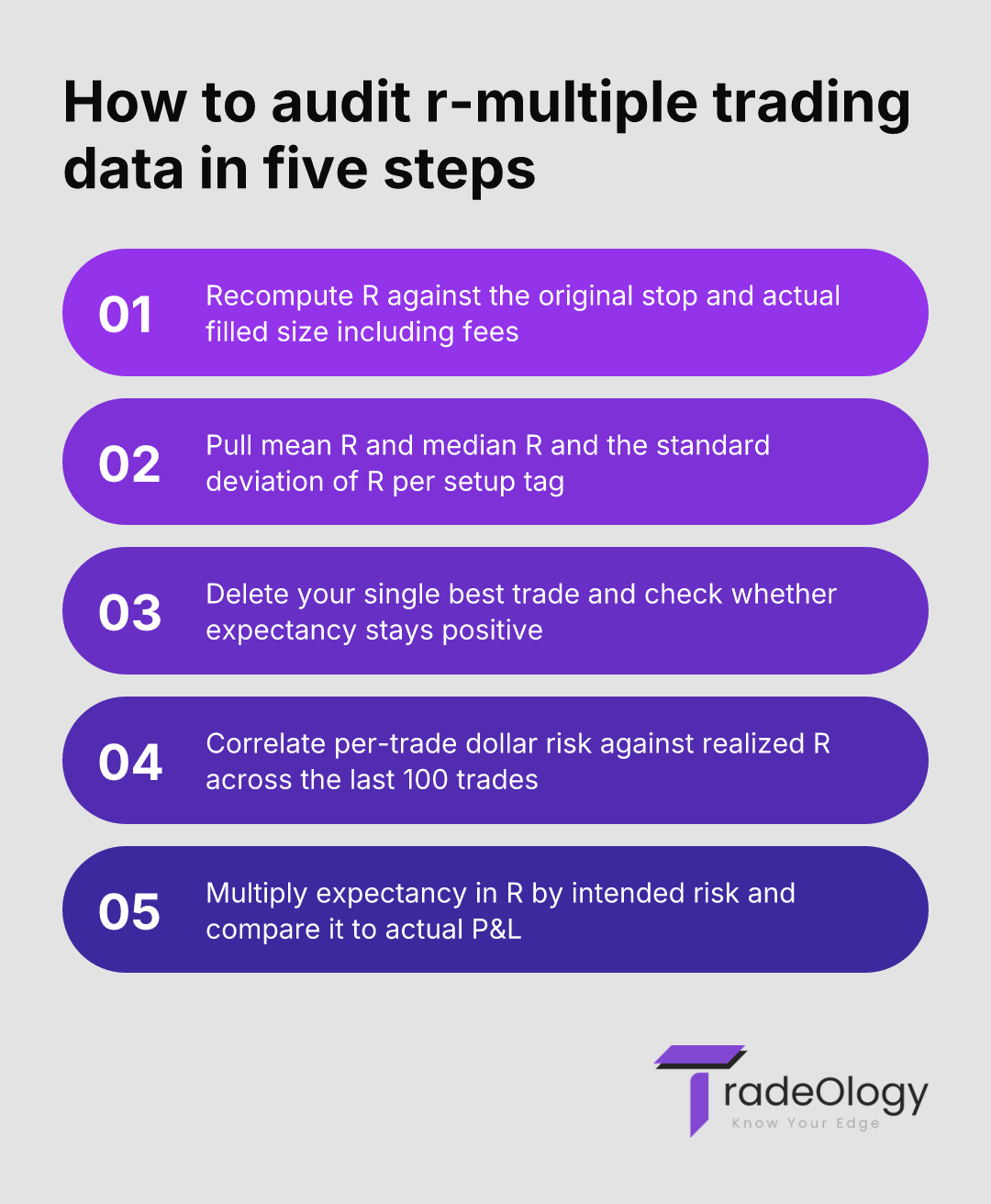
Fix the denominator. R must be computed against the risk on the executed entry — entry price minus original stop, times size, plus fees. Not the stop you wished you had used. Not the stop after you trailed it.
Rebuild the distribution. Pull mean R, median R, and standard deviation of R for the whole sample, then again per setup tag.
Test tail dependence. Remove your single best trade and recompute expectancy. If expectancy falls below zero, you have one lucky trade, not a system.
Correlate risk against R. Plot dollar risk on one axis and realized R on the other. A downward-sloping cloud is a sizing problem, and no setup refinement fixes it.
Convert back to dollars. Multiply expectancy in R by your intended constant risk and compare it to actual P&L. The gap is the cost of inconsistent sizing.
Setup checklist
Calculate R against the original stop and executed size on every trade, including scratches.
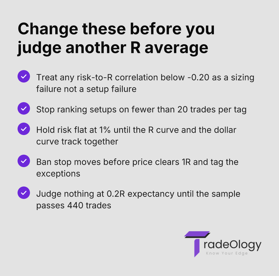
Compare mean R to median R per setup and flag any tag where the gap exceeds 1.0R.
Eliminate your single largest winner from the sample and re-run expectancy in R.
Analyze the correlation between dollar risk and realized R across the last 100 trades.
Tag every trade where you moved the stop before the first target and measure its mean R separately.
What each reading actually means
Metric | What it actually means | Action to take |
|---|---|---|
Mean R +0.4, median R -1.0 | Your edge is tail-driven and depends on a few runners. | Stop taking early partials and hold the sample to 300 trades. |
Positive expectancy in R, flat dollar P&L | Your largest positions are on your weakest trades. | Move to fixed fractional risk and re-measure over 50 trades. |
R standard deviation above 2.5 | Any average under 100 trades is inside the error bar. | Judge nothing until the sample clears 400 trades. |
Win rate up 8 points, mean R down 0.3 | Breakeven stops are converting winners into scratches. | Ban stop moves before price clears 1R. |
Drop best trade and expectancy turns negative | You are recording one outlier, not a repeatable process. | Keep risk at the low end until the pattern repeats. |
A worked example with real numbers
Account: $50,000. Intended risk: 1% per trade, so $500. Sample: 120 trades over five months, futures and stock momentum setups.
Reported R statistics: 38% win rate, average winner +2.6R, average loser -0.98R, expectancy +0.38R. Total: +45.6R. At a constant $500 of risk that is $22,800.
Actual P&L: +$3,100.
The reconciliation took ten minutes. The six trades above +4R carried an average risk of $210 — small size, taken hesitantly, on the setups the trader distrusted. The eleven full-stop losses in the same period carried an average risk of $1,150, all entered after two consecutive green days. Rank correlation between risk and R came out at -0.34.
Held at a flat $500, that same trade sequence returns roughly $22,800 before fees. The setup produced 45.6R of edge and the sizing handed back over 85% of it. This is why win rate obsession misses the point entirely — the win rate here was fine, the R distribution was fine, and the execution of size destroyed both.
If your expectancy in R is positive across 100 trades and your dollar P&L is not, stop refining the setup. Correlate per-trade dollar risk against realized R — if that number is negative, your sizing is eating the edge and every hour spent on entries is wasted.
Mistakes that corrupt the r multiple calculation itself
Recording R against the stop you should have used. A widened stop that survives becomes a fictional +2R instead of the real -1R plus a rule breach. Your log then rewards indiscipline.
Excluding scratches. A 0R trade is not neutral. It carries commissions, slippage and exposure, and a book full of them drags real expectancy below what your R average shows.
Blending holding periods. A +1.5R scalp and a +1.5R three-week swing are not comparable. Divide R by days held before you compare, or you will size the slow strategy as if it recycled capital weekly — the same distinction that matters when you price swing exposure per day.
Trailing stops into the denominator. Original risk defines R. Moving the stop changes the outcome, never the denominator. Confusing the two inflates every average you own.
Ranking setups on mean R with fewer than 20 trades per tag. With an R standard deviation above 2, a 15-trade tag tells you almost nothing about the setup and a great deal about the sequence.
Where TradeOlogy does the arithmetic for you
Reconstructing R-multiples by hand in a spreadsheet is the reason most traders never do it. TradeOlogy pulls executions from a connected brokerage account or a CSV import, groups them into round trips, and computes R per trade against the original stop and actual filled size — stocks, options, futures and crypto.
From there the useful views are the breakdowns. Expectancy in R per setup tag, per session and per hour, so you can see the histogram bar where mean R goes negative after 2pm. Distribution of R rather than a single average, so tail dependence is visible instead of assumed. And the dollar-versus-R gap, which is where the sizing problem shows up as an equity curve that lags the R curve. If you have never separated the two, start there — a trade log records what happened, while this tells you which half of your process is leaking. The free trial requires a card and you can cancel anytime.
FAQ
Why is my average R-multiple positive while my account is flat?
Because R-multiples normalise away position size. If your biggest dollar risk lands on your lowest-R trades, expectancy in R stays positive while dollar expectancy goes negative. Compute the correlation between per-trade risk and realized R; anything below -0.20 explains the gap without needing any other cause.
How many trades before an average R-multiple means anything?
It depends on the ratio of expectancy to the standard deviation of your R values. At 0.2R expectancy with a 2.1 standard deviation you need around 440 trades for the mean to sit two standard errors above zero. At 0.5R expectancy with the same dispersion, roughly 70 trades will do.
Does moving my stop to breakeven change the R-multiple calculation?
No. R is always measured against original risk at entry, so the denominator never changes. What changes is the numerator, and traders who move stops early typically add 5 to 8 points of win rate while losing 0.2R to 0.3R of mean R. Tag those trades and compare their expectancy against trades you left alone.
Should I record R-multiples on partial exits or the full position?
Record blended R for the whole round trip against the original risk, then log the partial separately as its own tag. Scaling out compresses the right tail of your R distribution, and if your strategy depends on 4R outliers, partials can turn a positive expectancy into a negative one while your win rate improves.
Can R-multiples compare two strategies with different holding periods?
Not directly. Divide expectancy in R by average days in trade to get R per day of exposure, then compare. A 0.3R day trade setup and a 1.2R six-week swing are close to equivalent per unit of exposure, and capital efficiency decides which one deserves the size.
Verdict
R-multiple trading data measures the quality of your setups and nothing else — it is size-blind by construction, which is precisely what makes it useful and precisely what makes it dangerous when read alone. Pair mean R with median R, the standard deviation of R, and the correlation between dollar risk and realized R. If those four numbers disagree with each other, your problem is sizing, not strategy, and no amount of entry refinement will change the P&L.